Downscaling module
Overview
High resolution crop allocation datasets are not usually available in open access sources. In principle, ‘downscaling models’ use high-resolution input data (e.g. in our case temperature, precipitation, soil pH etc.) which have predictive power over low-resolution input data (e.g. in our case national or admin level aggregate values of harvested area, production etc.).
In order to do so, we have used the Fine Scale Land Allocation Tool or FLAT model. FLAT is a statistical-based open access tool that combines dependent variable data measured at an aggregate level (e.g., state/provincial or national) with independent variable data measured at the pixel level to produce estimates of the dependent variable at the pixel level.
Input data preparation
In terms of the dependent aggregate values of harvested area, we have used FAO Agro MAPS Global Spatial Database of Agricultural Land use Statistics. The database provides agricultural statistics and data collected and compiled from national resources, surveys, and official in-country agencies, assuring some degree of consistency across different agricultural products and geographic areas. This consistency is considered highly important in this exercise as it allows replicability to other regions or agricultural products.
For the purposes of this exercise, level 2 administrative crop data were used as shown in Figure below.
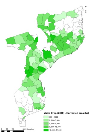
Visualisation of harvested area data of rainfed maize per admin level 2 in Mozambique, as retrieved from FAO Agro-Maps
Note
In case input data is outdated, they will need to be projected to the base year. For example in this case the total harvested area for maize was equal to only 782,608 ha in 2008 (input data), while 2017-18 FAO estimates indicate about 1,962,000 ha in Mozambique. This can be done through a python script available as Preparing Agro Maps.
Then, the above dataset is transformed into a base (vector) layer at the targeted downscaling resolution (e.g. 1km). This is used later on to extract the predictor attributes per location. The steps for this are as follows:
- Project crop layer to target crs (in this case EPSG: 32737 – WGS 84/UTM zone 37S )
- Calculate “area” in sq.km and “perimeter” in km for listed admin areas
- Convert “area” from sq.km to ha
- Create the base grid mesh (10km, 5km, 1km, 500m or 250m)
- Only keep locations where harvested area for the listed crop is available.
- Convert polygons to centroids indicating the location of crops at the selected resolution.
- Export output as a .csv file
Note
In order to facilitate the process, we have developed a QGIS plugin that together with instructions for installation and use is available at the project’s repository.
Finally, once base (vector) data layer is ready and available as a .csv file, predictor values are extracted from raster layers. As predictors in the FLAT model, we may use the following variables:
- Average temperature
- Average solar irradiation
- Average precipitation
- Average wind speed
- Soil Ph in H20
- Depth to bedrock
- Bulk density
- Clay content
- Texture class
- Soil organic carbon
- Drainage class
- EVI
- NDVI
- Elevation - Slope
- Cropland extent
The extraction process yields a .csv file that serves as input to the FLAT model. An example of this file is available as FLAT_input_Maize_10km.

Snapshot of the .csv file to be used as input in the FLAT model
Note
All of the above data can be collected either in their raw format or using a Python script (GEE_Imagery_Extraction) that was developed specifically for the extraction of the Images and ImageCollections using the GEE API.
Note
- The extraction process can be conducted through code available as FLAT prepping in the project’s repository.
- With regards to the imported geospatial layers (both raster and vector files), each one should be re-projected into the same coordinate system e.g. EPSG: 32737 – WGS 84/UTM zone 37S (+proj=utm +zone=37 +south +datum=WGS84 +units=m +no_defs) for Mozambique.
Parameterization & model run
The FLAT model can be executed with the following steps.
Step 1. Go to directory:
>/ FLAT_model/src
Step 2. In the directory run:
>/ Rscript RforFLAT.R flat_input.csv 0.534 1 15
where:
- flat_input.csv is the output csv of FLAT prepping process
- 0.534 is the target spatial resolution in arc.min
- 1 is the number of modelled crops
- 15 is the number of independent variables
Note
This process requires R to be installed at your working station. Running the above script creates nine derivative .csv files that are needed in Step 3. These include cropnames, pixels, states, data, statelevelcroparea, name, pixelarea, statelevelareainfo and variables.
Step 3. Copy the nine .csv files into the resource directory:
>/ FLAT_model/src/resource
Note
FLAT.gms should be located in the same directory as well - default by installation.
Step 4. Open GAMS Terminal; move to resource directory and run:
>/ gams FLAT.gms
Note
This will run FLAT model. Once complete, the log file (FLAT.ist) will be generated. This can be used to monitor the specifics of the run and track any issue in the debugging process (if needed). The result file is a .dat file usually under the name “finalresults.dat”. Other output files might include “Pixel-level cropland predictions against FAO aggregate values”; “Coefficient estimates”; ”Standard error”; “Covariate matrix for parameter estimation”.
Step 5. Export results (Optional)
>/ FLAT_model/src
run > Rscript dattotiff.R maize finalresults.dat (to generate a raster file (.tiff) of the results) or
run > Result.r (to export results in .csv format)
Note
Transformation of the result (.dat) file into a .csv file that can later on be used for the irrigation model can also be conducted using the script Dat to csv.
Output data
The output file provides a prediction the downscaled crop allocation. Each location (point in the vector layer) is attributed with a fraction of the total harvested area of the admin level it belongs to. Aggregation of the downscaled results per admin layer sum up to the original values.
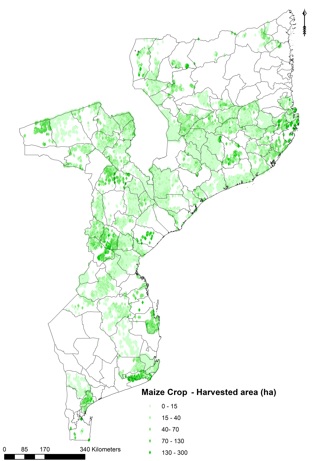
Example output from the downscaling process for rainfed maize in Mozambique
Special notes
The downscaling process is a good – yet experimental – way to achieve higher granularity of crop distribution, especially in areas where there is data scarcity.
The FLAT model that was selected in this assignment is open source (although GAMS is needed for big datasets) and straightforward to test, use and customize. It predicts cropland allocation using pixel-level biophysical attributes which are openly available at the desired spatial resolution (1 km). The econometric approach provides estimates of the effects of biophysical factors on cropland allocation.
FLAT performance metrics are in alignment with available literature; visual inspection of results does also agree with qualitative findings from sample agricultural survey. However, the selected cross-validation approach highlighted that inconsistencies in the sample dataset are high to achieve any satisfactory results. This highlights the need for standardization of collection, processing and dissemination of survey related datasets.
Note
A first and second order validation process was conducted in this project and is available in the project report. This was implemented through a Python script available as CrossValidation.